Assessment of German mortality until 2023

At the end of the battle the dead will be counted.

Destatis has released the official population statistic for 2023. A more precise calculation of mortality parameters becomes possible by that. Unlike raw death figures, population numbers in a current year must be estimated, but both are used to calculate mortality risks, which form the basis for other relevant indicators, such as life expectancy or mortality rates.

Error analysis

The development of the age cohorts starting from a known state can be computed week by week using the available death figures. In addition, the amount of people who die before they enter or leave a cohort, must be estimated. Unfortunately, this method is blind to immigration and emigration. The error of the age cohort populations at the end of 2023 was -1.6% in the 0-30 cohort, but dropped to negligible values ​​with increasing age (Fig. 1).

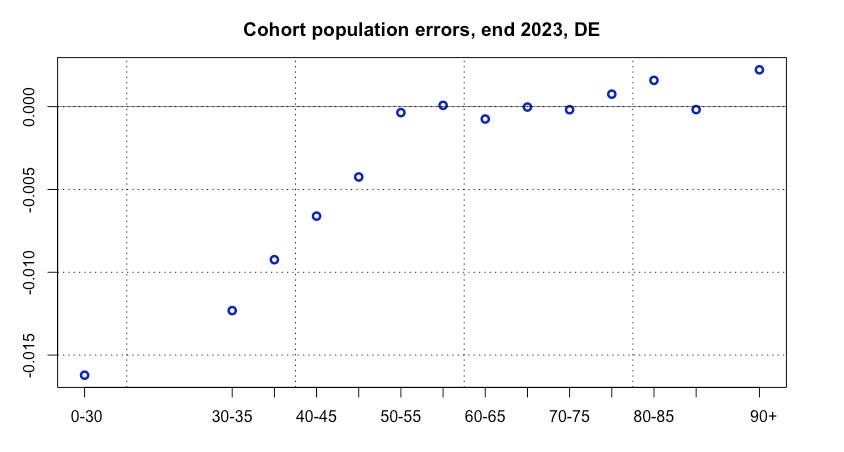
Fig. 1: Relative errors of German age cohort population.

Fortunately, errors in young cohorts have very little influence on the assessment of the general mortality, and viewed over the whole year, an averaging effect occurs, so that errors only count partly. The main results from previous articles concerning 2023 therefore remain valid.

Seasonality

2023 followed on in terms of seasonal oscillation. Until 2019, the seasonal maximum of deaths was reached in spring. In the years 2020-2023 it appeared phase-shifted to the early winter (Fig. 2). Although a four-fold repetition of an anomaly is quite extraordinary, it is currently unclear whether this observation has any meaning.

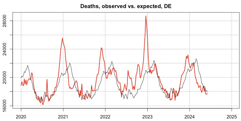
Fig. 2: Course of German deaths, observed (red) and expected (black).

Excess deaths

People often ask for excess mortality as a number, which says how many people have died more than normal. The problem here is to define what is normality. While effects caused by the aging of the society can simply be predicted, the risk trends in different age cohorts behave erratic. For example, the death risk of newborns substantially decreased during the past decades, meanwhile the risk at age 90+ has remained roughly constant.

Anyway, I took this approach and applied four different models to at least identify differences as well as similarities by comparison:

• Model 1: TSLM (Time Series Linear Model), trend + season, training period 2016-2020, forecast 2021-2024

• Model 2: TSLM, season only, training period 2016-2020, forecast 2021-2024

• Model 3: Exponential long-term trend, training period 2011-2020, forecast 2021-2024

• Model 4: ARIMA [1,1,0], training period 2011-2020, forecast 2021-2024

In all models, the development of death risks is analyzed separately in 14 age cohorts, which are determined in the current weekly reports. Deaths and cohort populations are collected weekly to calculate, fit and forecast the cohort risks. Multiplying the expected risks by the population numbers finally yields an estimate of expected deaths for each week in each age cohort. The annual cumulative differences between the reported and predicted death numbers represent the excess mortality shown in Fig. 3.

           year  Excess deaths   percentage

Model 1    2020           5000        0,5 %
           2021          36000        3,6 %
           2022          74000        7,4 %
           2023          26000        2,6 %
           2024         -20000       -4,2 %
            
Model 2    2020          -2000       -0,2 %
           2021          26000        2,6 %
           2022          59000        5,9 %
           2023           8000        0,8 %
           2024         -29000       -6,2 %
            
Model 3    2020           4000        0,5 %
           2021          36000        3,7 %
           2022          75000        7,6 %
           2023          28000        2,8 %
           2024         -21000       -4,5 %
            
Model 4    2020           6000        0,6 %
           2021          36000        3,6 %
           2022          73000        7,4 %
           2023          25000        2,5 %
           2024         -21000       -4,5 %

Fig. 3: Annual excess deaths of four different models. Figures for 2024 up to calendar week 23.

Model-caused differences are not surprising. Nevertheless, a consistent pattern emerges. Starting from the year 2020 that can be classified as almost normal, excess deaths rose in 2021, peaking in 2022, which in the most conservative “Model 2” amounted to 59k. In 2023, three models still detect a moderate excess mortality, which has been nearly compensated in the weeks available so far for 2024.

Trends depending on age

As mentioned above, the risk trends differ depending on age. This can be demonstrated by risk ratios, i. e. the risk in a specific year and age cohort in relation to the predicted risk of the same age cohort at the same time. I applied “Model 2”, which ignores the trend term and got the diagrams in Fig. 4.

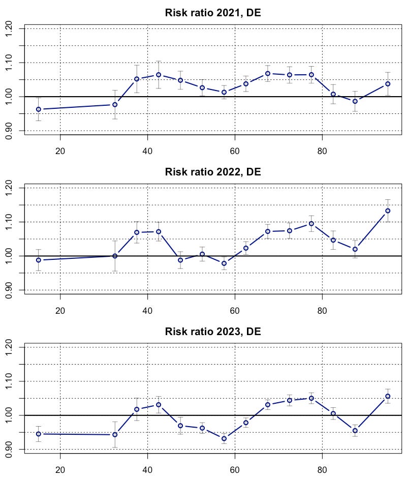
Fig. 4: Risk ratios on the base of “Model 2” with 95%CI.

The cohorts 45-65 show a remarkable commonality. Their risk ratios are steadily decreasing. To take a closer look, I extracted the trends and related p-values from “Model 1”, which in contrast to “Model 2” postulates a trend term (Fig. 5).

cohort       trend   p-value   significance  
      
  0-30    -0.02663   0.00000   yes
 30-35    -0.02522   0.00016   yes 
 35-40     0.00721   0.17416   no
 40-45    -0.00369   0.43276   no
 45-50    -0.01612   0.00000   yes 
 50-55    -0.01838   0.00000   yes 
 55-60    -0.01858   0.00000   yes 
 60-65    -0.00617   0.00639   yes 
 65-70     0.00173   0.45779   no
 70-75    -0.00282   0.32073   no
 75-80     0.00764   0.01117   yes
 80-85    -0.01206   0.00050   yes 
 85-90    -0.00727   0.07042   no 
   90+     0.00774   0.08892   no 

Fig. 5: Relative risk trends p. a. in 14 age cohorts, p-values and significance from “Model 1” (training period only).

Actually, a clear negative trend in the cohorts 45-65 is revealed. At both sides, this group is framed by two cohorts with weak and non-significant trends. In Fig. 4 we also found a continuation of this trend until 2023. So an ongoing process is identified. The other cohorts behave differently. While the older cohorts showed weak and partially insignificant trends, certain changes are found in the youngest two cohorts. This is probably an artifact of accident avoidance in 2020, and should not be overestimated, especially since the confidence intervals for younger people are quite large.

Life expectancy

Let's watch the situation from a different angle, namely life expectancy at birth, a very reliable indicator of overall societal mortality. I calculated LE values for every single week since 2000 and implemented several trend lines (Fig. 6).

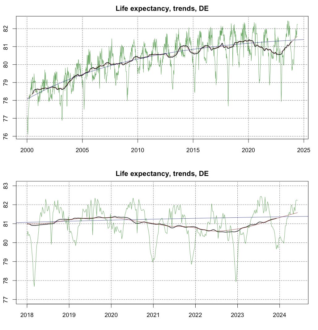
Fig. 6: German weekly LE (green) with exponential long-term trend (blue), STL-trendcycle (red) and 52-week moving average (black).

The shorter-term trend lines have been moving away from the long-term trend line since 2020 forming a gap of historical intensity and duration. The turning point is located in 2022. Since then, there has been a gradual convergence with the long-term estimates. The red line from the STL decomposition has even crossed the blue one at early 2024. An interesting detail should also be noted. All-time highs were set during several summer weeks in 2023, even though this year only achieved 4th rank overall. If only the first 23 calendar weeks are considered, 2024 takes the first place.

Summary

Some indicators point to a normalization of the death rates in Germany. Some trends of the past seem to continue now, as far as they became visible. On the other hand, unusually high levels of incapacity to work due to illness were reported last winter and spring. Morbidity may behave quite differently from mortality in this case.

I would not yet describe the situation as completely normalized. From Fig. 6 you can see that in previous years the blue long-term trend line frequently has been exceeded for many months or even years by the black and red lines. This has not yet been occurred.

So I will continue counting the living and the dead for a while…