


Longevity trends in German life expectancy: Where do we stand with 2023?
The trend is your friend.

It is one thing to determine life expectancy at birth (LE) or mortality rates from available death counts and population data - but quite another to judge them fairly, if they are drifting towards unusual directions.
The extrapolation of values from the past requires a well-founded hypothesis regarding the underlying long-term development. If periods are directly compared, underlying trends are neglected. If periods are compared with the assumption of linear trends, curvatures of the trend may be neglected. The LE in Germany belongs to this category (Fig. 1).

Fig. 1: Life expectancy at birth, 2000-2023
The trend can be seen very clearly in the development since 2000. The flattening slope of the trend line shows a picture that is familiar to every engineer. It is the step response of a so-called 1st order lag system, also known as low-pass filter. It can be described by the equation
y = A - B*exp(-C*x)Another argument for an exponential damped trend is that this type of function is a valid standard in actuarial sciences.
These considerations lead to a result that contrasts with the frequently expressed assumption that LE can be increased further and further. According to the current data, it will reach a natural barrier at 81.8 years as long as no decisive improvements come in sight e. g. in the treatment of life-threatening mass diseases.
Official data on LE is usually given in single-year or multi-year averages. This is far too rough for detecting short-term developments. However, LE can also be determined from the weekly mortality data published by Destatis in 14 age cohorts. The age cohorts must be converted to age year groups and the population status must be estimated weekly or monthly - challenging, but feasible with minor errors, as the comparison with official data from the past has shown.
This way a weekly time series of LE is obtained. I applied a STL decomposition to separate the seasonal part and the trend part and executed a non-linear parameter estimation on the latter. The following R-print provides information about the quality of the fit over the period 2000-2020.
Formula: y ~ A - B * exp(-C * x)

Parameters:
     Estimate  Std. Error t value            Pr(>|t|)
A 81.78144431  0.01586294 5155.50 <0.0000000000000002 ***
B  3.61572373  0.01300636  278.00 <0.0000000000000002 ***
C  0.00183967  0.00001911   96.25 <0.0000000000000002 ***
---
Signif. codes:  0 ‘***’ 0.001 ‘**’ 0.01 ‘*’ 0.05 ‘.’ 0.1 ‘ ’ 1
Since the p-values of all three parameters are several orders of magnitude below the 5% level of significance, they can be trusted with a high degree of certainty.
Modern time series methods such as ARIMA can map curvatures and minimize autocorrelations, but tend to produce systematic trend errors in signals of the given characteristics. I checked this out by feeding them with a hypothetic series according to the equation
y = A - B*exp(-C*x) + |D*sin(x)| + noiseHowever, the trend now becomes predictable for a few years, and by superposing the seasonal pattern you get a pretty week-by-week fit and point forecast (Fig. 2, black line).
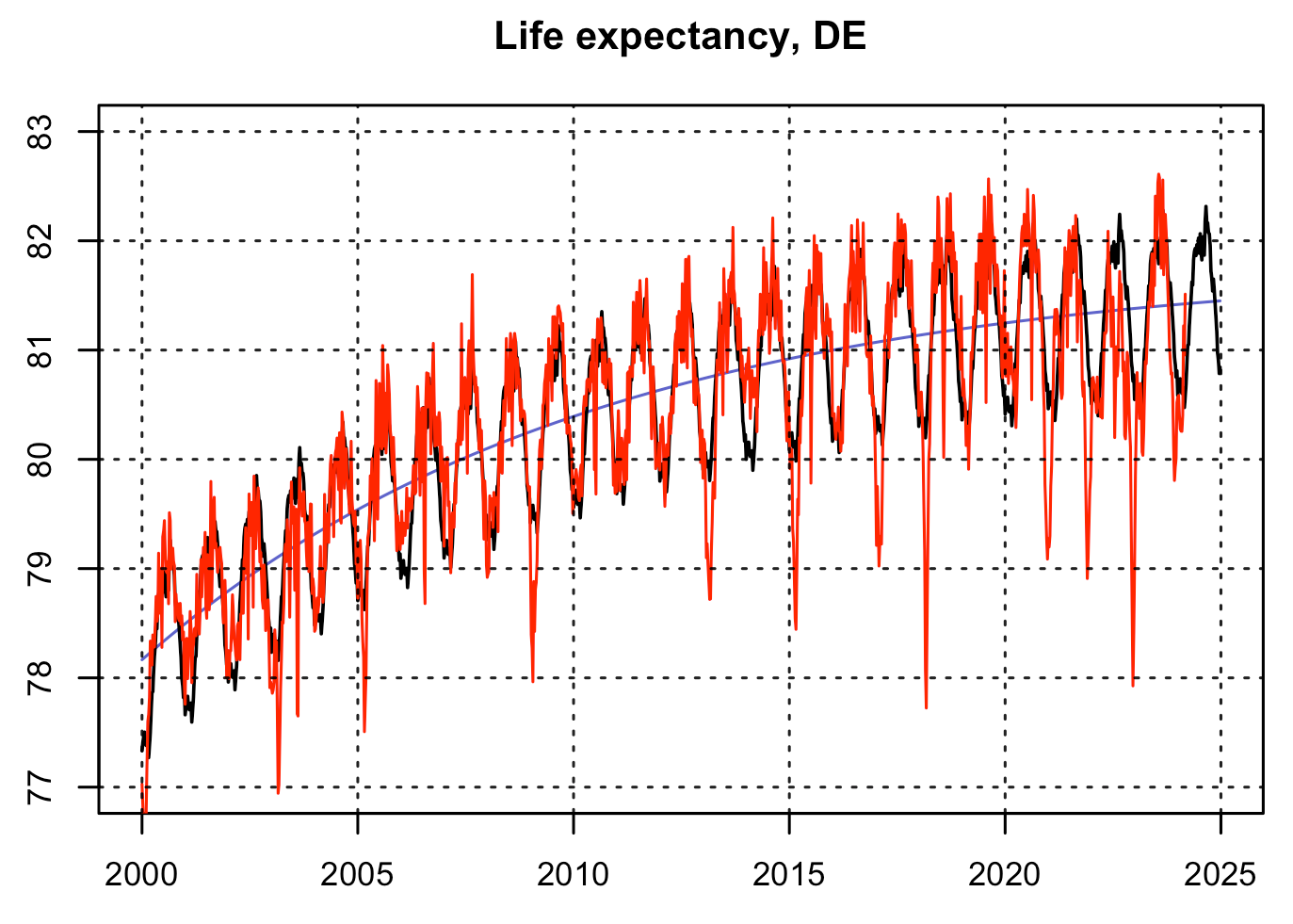
Fig. 2: Seasonal LE, observed (red), trend (blue), model fit and forecast (black)
The enlarged detail since 2019 shows the meanwhile well-known patterns of excess mortality with deep notches at the end of the years and vast difference areas between expected and observed values from mid 2021 to late 2022 (Fig. 3, 4).

Fig. 3: Loup from Fig. 2. The values for 2024 should be considered provisional with decreasing tendency due to late registrations.
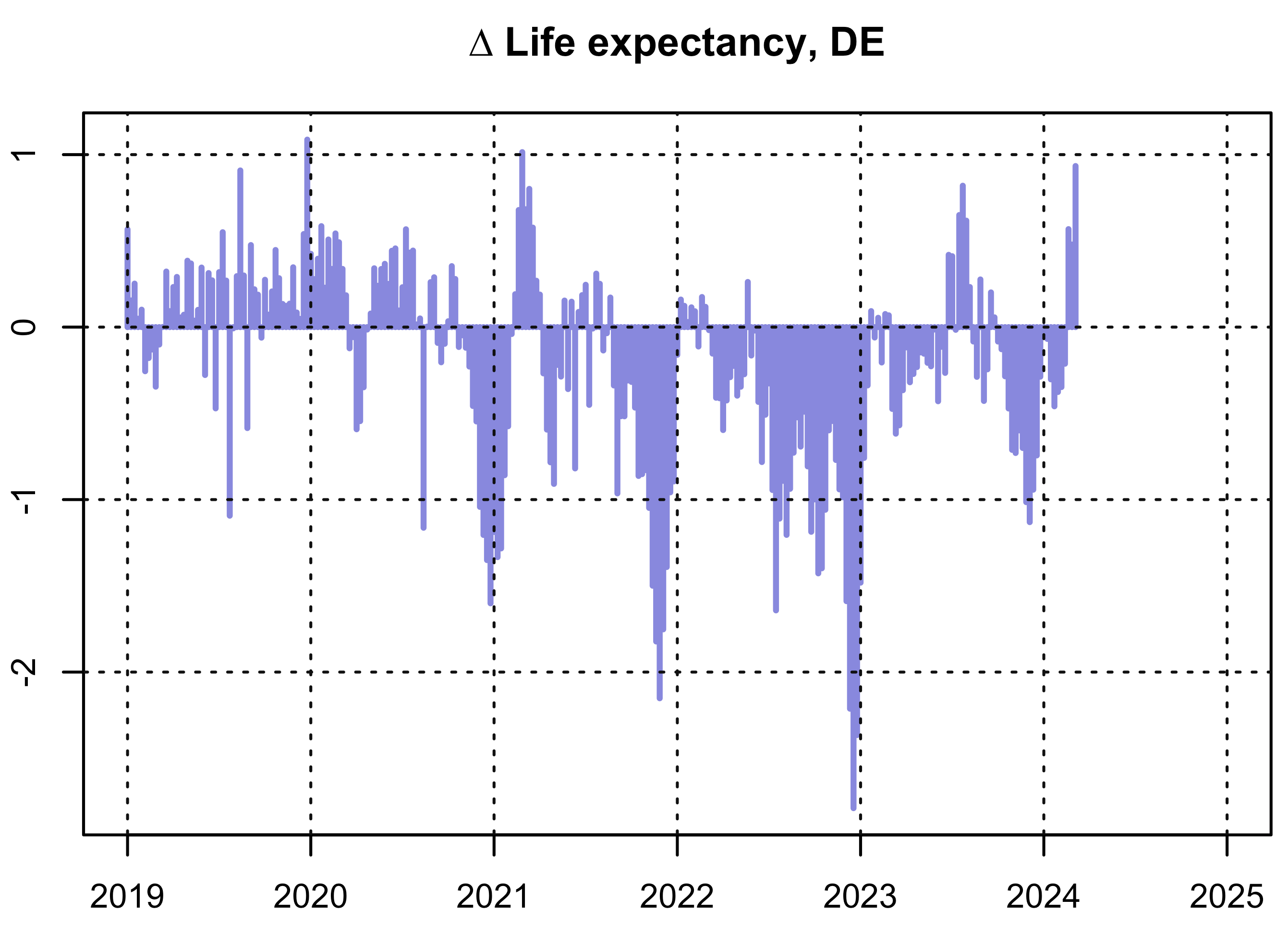
Fig. 4: Deviations of LE, observed - expected.
The cumulative sum of the deviations is also very suitable for assessment (Fig. 5).

Fig. 5: Cumulated differences of LE, observed - expected
The all time high year in LE was 2019. Starting from this high level, the differences continued to increase for a while. At the end of 2020, the differences had come down to almost zero, just as was constantly observed in the pre pandemic era. It must be stated clearly that the pandemic threat in 2020 was purely imaginary. Hardly any other analysis can reflect this fact so convincingly.
The following years 2021-2023 accumulated a difference in LE of around -60 years. To fully understand this result, we must remember that the differences were added up weekly. Therefore -60 years correspond to a lifetime loss of one year for a period of 60 weeks. Admittedly, this seems very abstract to most people, who ask then for excess deaths (ED) or percentage excess mortality. I asked myself whether the loss of LE (dLE) can be converted into ED, at least approximately. The high level of certainty of trend prediction would be a strong argument for such a calculation.
Because both, mortality and LE depend on the age-specific risk of death r, the question can be varied: How are dLE and the relative change in the common risk of death (dr) related? To answer this, I extracted the gradient s = dr/dLE from the LE calculation model. I assumed that dr would be limited between 3% and 7%, what I consider to be a realistic scale for a yearly variation. It turns out that s varies slightly (error < 1%) and for the typical value dr=5% it is s = 0.1153. In short, an increase of mortality risks of dr=11.53% corresponds to a 1-year-drop of LE. Data source was the German lifetable 2018-2020.
We also know the average weekly deaths in the epoch 2018-2020 of 18,400 and finally obtain the wanted yearly excess deaths:
    47,000 ED in 2021
    73,000 ED in 2022
    22,000 ED in 2023
   ------------------
   142,000 ED in 2021-2023
In addition, it can be said that ED in 2020 ranked below the noise level at approximately zero, which was to be expected since LE was close to the expected value. Comparable findings are provided by another model that determines the risk trends separately from the 14 age cohorts during the reference epoch 2011-2020:
    37,000 ED in 2021
    76,000 ED in 2022
    27,000 ED in 2023
   ------------------
   140,000 ED in 2021-2023
Unfortunately, the model outcomes drift when the reference period is extended to 2000-2020. Apparently the long-term trends of individual cohorts are determined unreliably due to trend breaks in some age cohorts.
Other authors, for example Kuhbander and Reitzner recently published slightly lower numbers which, however, point to the same direction. An uncertainty of ±10,000 (approx. ±1%) can be considered normal for the German ED as a consequence of different methods and the assumptions and neglects they presuppose.
The question posed in the title can now be answered clearer. 2023 has to be assessed in connexion with the previous years. As already 2021 and 2022, 2023 also ended with excess mortality. Three consecutive years of excess mortality i. e. loss of LE are unique in the time series. If a year falls below the trend line, a significant compensation or even overcompensation usually occurs in the following year. The last quarter was primarily responsible for the negative performance. A connection with the booster campaign launched in autumn is conceivable, but maybe an insufficient explanation. In addition, from autumn onwards there was a very high level of sickness due to respiratory infections.
2023 also followed on from previous years in terms of seasonal oscillation. Until 2019, the minimum life expectancy was in calendar week 9. In the years 2020-2023 it appeared phase-shifted to calendar week 51 (Fig. 6). It is currently completely unclear whether this anomaly has any meaning.

Fig. 6: Average seasonal oscillation, 2000-2019 (green), 2020-2023 (red), x-axis: calendar weeks
It should be mentioned that in summer 2023 inconspicuous values were achieved. In the weeks 29 and 31 the best weekly values of all time were measured. The weeks 34 and 28 got rank 4 and 5.
Isn’t it funny that at this time, the Robert Koch Institute officially installed a climate monitoring to draw attention to the danger of deaths due to heat stress?
That reminds me of something. The same thing again, in 2023 as in 2020. When LE looks pretty good, lobby lackeys seem to start spreading fear under an arbitrary pretext.